Understanding the nuances of transformer inference is crucial for optimizing performance and cost. In this blog, we will delve into key concepts such as arithmetic intensity, memory bandwidth, and GPU throughput, going through critical calculations for transformer models like LLaMA 2 on A10 GPUs. We'll explore how to estimate different performance-bound scenarios—whether your model is memory, compute, overhead, or communication-bound—and present strategies for optimizing cost and latency. By the end, you'll have a framework for making informed decisions on how to best utilize your GPU resources for high-throughput transformer inference and a theoretical estimator app comparing costs and performances across different GPUs.
Understanding GPU spec :
Calculate the operations-to-byte (ops:byte) ratio of your GPU from its specifications. For A10 GPU spec:
ops_to_byte_A10
    = compute_bw / memory_bw
    = 125 TF / 600 GB/S
    = 208.3 ops / byte
Understanding Transformer Inference Calculations:
- The most computationally expensive part of transformer inference is the attention layer.
- To calculate the arithmetic intensity (operations per byte) of the attention layer, we need to break down the attention equation: $Attention(Q, K, V) = softmax(QK^T/sqrt(d_k))V$
- Let N be the sequence length, d be the dimension of a single attention head, Q, K, and V be matrices of size N by d with fp16/bf16 precision.
- The total compute in floating point operations is approximately: $4(N^2)d + 3N^2$
- Attention Calculation ($A = QK^T$): $2(N^2)d$ FLOPs - $Q$ and $K$ have dimensions $N \times d$, and their dot product requires $2N^2d$ floating point operations.
- Softmax Operation $A = softmax(A)/sqrt(d_k)$: $3N^2$ FLOPs - The attention matrix $A$ has size $N^2$. Calculating the exponent for each element requires $N^2$ FLOPs, and the normalization (sum and division across rows) requires an additional $2N^2$ FLOPs.
- Output Calculation $O = A.V$: $2(N^2)d$ FLOPs - $A$ is of size $N \times N$ and $V$ is $N \times d$. The dot product between $A$ and $V$ takes $2N^2d$ FLOPs.
- The total memory movement in bytes is approximately: $8N^2 + 8Nd$
- Attention Calculation $A = QK^T$: $4Nd + 2N^2$ bytes - $Q$ and $K$, each of size $N \times d$, require $2Nd$ bytes each in FP16 precision. The resulting attention matrix $A$, of size $N^2$, takes $2N^2$ bytes.
- Softmax Operation $A = softmax(A)/sqrt(d_k)$: $4N^2$ bytes - The input and output of the softmax operation, both of size $N^2$, require $2N^2$ bytes each in FP16.
- Output Calculation $O = AV$: $2N^2 + 4Nd$ bytes - The attention matrix $A$ of size $N^2$ requires $2N^2$ bytes, and the vectors $V$ and output $O$, both of size $N \times d$, require $2Nd$ bytes each.
- The arithmetic intensity is then calculated as: arithmetic_intensity = $(4(N^2)d + 3N^2) / (8N^2 + 8Nd)$
- For Llama 2 7B, the arithmetic intensity is around 62 operations per byte.
Estimating 4 types of Bound Scenarios:
Compare the ops:byte ratio to the arithmetic intensity of your model.
- Memory Bound: If the arithmetic intensity is lower than the ops:byte ratio, the model is memory bound (limited by memory bandwidth).
- Compute Bound: If the arithmetic intensity is higher than the ops:byte ratio, the model is compute bound (limited by compute resources).
- Overhead Bound: In dynamic languages like PyTorch, the overhead of converting code into GPU execution instructions can sometimes exceed the time spent on execution itself. In such cases, tools like
torch.compileor Triton can optimize the execution by reducing overhead. - Communication Bound: When a significant amount of time is spent on communication between devices, the model is communication-bound. This typically occurs in distributed computing environments.
For Llama 2 7B on an A10 GPU, the model is memory bound during autoregressive sampling (arithmetic intensity of 62 ops/byte < 208.3 ops/byte).
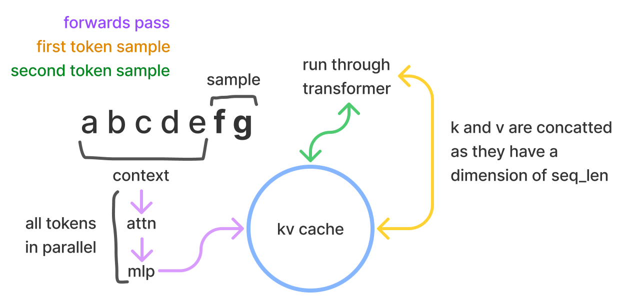
KV cache and batch size estimation
Remaining VRAM = 24 GB - (2 * 7GB) = 10GB # 2 A10 GPU with 12GB VRAM

kv_cache_size
    = (2 * 2 * n_layers * d_model) bytes/token
    = (4 * 32 * 4096) bytes/token
    = 524288 bytes/token
    ~ 0.00052 GB/token

kv_cache_tokens
    = 10 GB / 0.00052 GB/token
    = 19,230 tokens

batch_size = 19,230/2048 = ~9  => Batch size of 8 can be supported over context len of 2048.
Estimating Cost and Latency:
Prefill time = number of tokens * ( number of parameters / accelerator compute bandwidth)
time/token = total number of bytes moved (the model weights) / accelerator memory bandwidth
Total generation time = prefill time + number of tokens * time/token
For A10, llama 7B models:
prefill_time = 350 * (2 * 7B) FLOP / 125 TFLOP/s = 39 ms
time/token = (2 * 7B) bytes / (600 GB/s) = 23 ms/token
Total Generation Time = 39 ms + 150 tokens * 23 ms/token = 3.49 s
For example, on 2 A100 GPUs with a batch size of 1 for Llama 7B, the estimated cost is $0.066 per 1K tokens, which is higher than GPT-3.5's cost.
Increasing the batch size can reduce the cost but may increase latency.
Model Bandwidth Utilization (MBU):
- MBU measures what percentage of the GPU's memory bandwidth is being utilized during inference.
- It is calculated as:
(model_size_in_bytes * tokens_per_second) / GPU_memory_bandwidth - Higher MBU indicates better utilization of the GPU's memory bandwidth capabilities.
- The above token time estimates are with 100% MBU but in typical experiments, 70% MBU is achieved. These numbers can be scaled to match more real-world scenarios.
Optimizing Performance:
- Batching: Run forward passes through the model in batches to reuse parts of the model loaded into GPU memory, increasing arithmetic intensity.
- Quantization: Use lower-precision quantization (e.g., INT8, INT4) to reduce the memory bandwidth required for loading model weights.
- Speculative Decoding: Use a smaller "draft" model to generate tokens quickly, then verify them with the larger "verifier" model, reducing the number of times the larger model's weights need to be loaded.
- Tensor Parallelism: Split the model across multiple GPUs to leverage more memory bandwidth and compute resources, improving latency.
- Kernel Optimization and Compilation: Tools like torch.compile can generate highly optimized kernels for operations like matrix multiplications and attention, sometimes outperforming hand-tuned libraries like cuBLAS and FlashAttention.
- Communication Overhead: Communication overhead between devices, like during model parallelism, can be a significant bottleneck and should be accounted for in performance estimations.
Awesome Resources
- GPU specs - Calculating the operations per byte (ops:byte) ratio
- LLM - Calculating arithmetic intensity
2.1 Prefill: Prompt processing (processing the input tokens) is compute-bound and relatively inexpensive compared to token generation.
2.2 Autoregressive sampling: Token generation is memory-bound, as it requires loading the model weights for each generated token, making it more expensive. - KV cache and supported batch size estimation.
- Token Generation Time Estimation
- Cost Estimations
Roofline Paper - understanding performance measurement

Other techniques like Grouped Query Attention, MOE, Paged Attention, Flash Attention, Prefix caching etc improve LLM performance. -> these can be added to corresponding bound scenarios to as improvement examples.
Here is a simple cost estimator with defaults for the Llama 70B model with 8 CB factor (due to Grouped Query Attn) and achieved GPU utilisation (MFU) of 70%. (Colab Notebook Reference)
GPU Cost Calculator
During the training of deep neural networks, the mean and variance of activations can quickly shoot off to very high values or drop down to zero, causing the local gradients to become NaN or zero. This prevents the network from learning effectively. There are
]]>
During the training of deep neural networks, the mean and variance of activations can quickly shoot off to very high values or drop down to zero, causing the local gradients to become NaN or zero. This prevents the network from learning effectively. There are several techniques to handle this vanishing/exploding gradient problem:
- Proper Weight Initialization: Initialization methods like Xavier/Glorot or Kaiming/He scale the weights based on the number of input and output units, ensuring that the variance of the activations is preserved across layers. It helps prevent the activations from exploding or vanishing in the initial stages of training.
- Gradient Clipping: It clips the gradients to a maximum value during backpropagation to prevent them from becoming too large. It improves stability during training and can be applied to the gradients of individual parameters or the global norm of the gradients.
- Batch Normalization: Batch/Layer Normalization is a widely used technique that normalizes the activations of each layer to have a mean of zero and a standard deviation of one. It also acts as a form of regularization, improving the model's generalisation performance.
- Activation functions: Using activation functions that have non-vanishing gradients, such as ReLU (Rectified Linear Unit) or its variants (Leaky ReLU, ELU), can help mitigate the vanishing gradient problem. activation-functions-explained
- Model Architecture: Residual connections, as used in ResNet architectures, provide an alternative path for the gradients to flow through the network. LSTM/GRU address the vanishing gradient problem in traditional recurrent networks.
- Advanced Optimisers: Optimisers like LARS, LAMB or LION help to mitigate the exploding gradient problem by adjusting the learning rates dynamically during training. A proper warmup schedule also helps in achieving learning stability.
Although, there are multiple approaches, good initial parameters are very essential. Along with other techniques, a good initialization improves training efficiency, resulting in better models at lower cost.
Common Initialization Strategies
Zero Initialization
Setting all weights and biases to zero is a bad strategy as it prevents symmetry breaking and halts gradient flow.
Random Initialisation
Initializing weights with random numbers from a normal distribution can help break symmetry, but the activations still tend to diminish or explode for deeper layers.
Xavier/Glorot Initialization
Proposed in 2010, this initialization scales the weights by $\sqrt{1/n}$, where $n$ is the number of input units. It helps ensure that the variance remains the same across layers for tanh/sigmoid activations.
Where 𝑈 is a uniform distribution and 𝑓𝑎𝑛𝑖𝑛 is the size of the previous layer (number of columns in 𝑊) and 𝑓𝑎𝑛𝑜𝑢𝑡 is the size of the current layer.
Kaiming/He Initialization
For ReLU activations, Xavier initialization is not optimal. Kaiming initialization scales the weights by $\sqrt{2/n}$, which helps maintain the variance across layers. This implies an initialization scheme of:
𝑤𝑙∼𝑁(0,2/𝑛)
That is, a zero-centered Gaussian with a standard deviation of 2/𝑛 (variance shown in equation above). Biases are initialized at 0.
LSUV Initialization
Layer-Sequential Unit-Variance Initialization ( All you need is a good init) is a simple method for weight initialization for deep net learning. The initialization strategy involves the following two-step:
- First, pre-initialize weights of each convolution or inner-product layer with orthonormal matrices.
- Second, proceed from the first to the final layer, normalizing the variance of the output of each layer to be equal to one.
Fixup and T-Fixup Initialization
FixUp Initialization, or Fixed-Update Initialization, aims to train very deep residual networks stably at a maximal learning rate without normalization. It fixes the variance scaling issue due to residual connection. Initialize with Kaiming enable stability after activation: ie $Var(F(x))=Var(x)$ . But now with residual $Var(F(x)+x)$ will be greater than $ Var(x) $ so variance grows with each block!
The steps are as follows:
- Initialize the classification layer and the last layer of each residual branch to 0.
- Initialize every other layer using a standard method, e.g. Kaiming Initialization, and scale only the weight layers inside residual branches by $L^{\frac{1}{2m-2}}$.
- Add a scalar multiplier (initialized at 1) in every branch and a scalar bias (initialized at 0) before each convolution, linear, and element-wise activation layer.
Setting weights to zero can result in the problem of gradient flow halting and symmetricity breaking. The Fixup initialization strategy addresses issues in deep residual networks by utilizing residual connections. These connections allow gradients to flow uninterrupted through the network, preventing vanishing gradients and ensuring continuous learning. Additionally, Fixup breaks symmetry by initializing the first convolutional layer with a non-zero method, enhancing the diversity of learned features. This asymmetry propagates through the network via residual connections, further boosting the model's representational power.
T-Fixup extends this concept further to transformer models.
Calculating Fan-in and Fan-out
For dense layers, fan-in is the number of inputs, and fan-out is the number of outputs. For convolutional layers:
fan_in = num_input_feature_maps * receptive_field_size
fan_out = num_output_feature_maps * receptive_field_size
PyTorch Implementation
PyTorch does not use modern initialization techniques by default for backward compatibility reasons. You can explicitly initialize the weights using torch.nn.init functions for proper initialization:
import torch
import torch.nn as nn

# Helper function for initializing weights
def init_weights(m):
    if isinstance(m, nn.Conv2d) or isinstance(m, nn.Linear):
        # Kaiming initialization for convolutional and linear layers
        nn.init.kaiming_normal_(m.weight, mode='fan_out', nonlinearity='relu')
        if m.bias is not None:
            nn.init.constant_(m.bias, 0)
        if hasattr(m, 'special_init'):
            nn.init.constant_(m.weight, 0)
    elif isinstance(m, nn.BatchNorm2d):
        # Batch normalization layer initialization
        nn.init.constant_(m.weight, 1)
        nn.init.constant_(m.bias, 0)

# Example model
class ExampleModel(nn.Module):
    def __init__(self):
        super(ExampleModel, self).__init__()
        self.conv1 = nn.Conv2d(3, 32, kernel_size=3, padding=1)
        self.bn1 = nn.BatchNorm2d(32)
        self.conv2 = nn.Conv2d(32, 64, kernel_size=3, padding=1)

        # Flag the 2nd convolutional layer for special init
        self.conv1.special_init = True


    def forward(self, x):
    	...


# Initialize the model weights
model = ExampleModel()
model.apply(init_weights)
Different initialization strategies are suitable for different activation functions and network architectures. Understanding the rationale behind these strategies will help you improve your networks efficiently. To learn more about this, these are some good references:
]]>In our previous blog, we delved into the implementation and training of a GPT-based transformer model, incorporating several minor optimizations. The transformer architecture has showcased remarkable resilience to evolving trends. Beyond the PreNorm technique, another critical area that researchers have significantly improved is positional encoding. Positional encoding enables the model to comprehend the relative positions of words within a sentence, a vital factor for tasks like language translation and text generation.
The introduction of new positional embedding methods has empowered models to effectively capture larger contextual information. It has also served as a foundational element in various Language Model (LLM) architectures, including T5, Llama, and MPT.
In this post, we'll delve into the evolution of positional encoding techniques and their integration into transformer models. The final section offers a summary and comparison of these methods. You can practice these concepts by following the linked Colab Notebook, featuring step-by-step code implementation.
Hands-on Notebook: github
Experiment Dashboard: wandb
Vanilla Transformer Model
The vanilla transformer model, introduced by Vaswani et al. in 2017, uses a sinusoidal function to encode the position of each word in the input sequence. This positional encoding is added to the word embeddings before being fed into the model. The sinusoidal function has the advantage of being able to represent an arbitrary length sequence, but it has some limitations in terms of expressiveness. Authors also experimented with using learned positional embeddings but found no significant impact. So sinusoidal-based positional encoding was selected.
Integrated Positional Embedding
In later studies, it was discovered that learned positional embedding had no advantage because positional embeddings were just added initially. In deep multilayered networks, positional embedding goes through so much transformation that positional information is rendered ineffective. To improve the expressiveness of positional information in the entire network, positional information is integrated into each transformer block in the model. This involves learning a separate embedding for each position in the input sequence, for every transformer block. Integrated positional embedding has been shown to improve performance, but it has the disadvantage of requiring a fixed maximum sequence length.
We can incorporate absolute position into embedding space as:
where P is the position embedding vector. This can be incorporated in MHSA implementation as follows:
class MultiHeadAttention(nn.Module):

    def __init__(self, num_heads, head_size, shared_head=False):
        super().__init__()
        self.num_heads = num_heads
        self.head_size = head_size
        self.shared_head = shared_head

        self.key = nn.Linear(head_size, head_size, bias=False)
        self.query = nn.Linear(head_size, head_size, bias=False)
        self.value = nn.Linear(head_size, head_size, bias=False)
        self.register_buffer('tril', torch.tril(torch.ones(block_size, block_size)))

        if self.shared_head:
          self.pos_emb = nn.Parameter(torch.randn(block_size, head_size))
        else:
          self.pos_emb = nn.Parameter(torch.randn(num_heads, block_size, head_size))

        self.dropout_wei = nn.Dropout(dropout)
        n_embd= num_heads*head_size
        self.proj = nn.Linear(n_embd, n_embd)
        self.dropout_proj = nn.Dropout(dropout)


    def forward(self, x):
        # Reshape the tensor to B N T H for N heads
        B,T,C = x.shape
        x = rearrange(x, 'B T (N H) -> B N T H', N=self.num_heads)

        k = self.key(x)   # (B,N,T,H)
        q = self.query(x) # (B,N,T,H)

        # compute attention scores
        q = q * self.head_size**-0.5
        wei = torch.einsum("BNTH, BNSH -> BNTS", q,k)

        # Position Embedding
        if self.shared_head:
          p_wei = torch.einsum("BNTH, SH-> BNTS" ,q,self.pos_emb[:T])
        else:
          p_wei = torch.einsum("BNTH, NSH-> BNTS" ,q,self.pos_emb[:,:T,:])

        wei += p_wei

        # final attention and value computation
        wei = wei.masked_fill(self.tril[:T, :T] == 0, float('-inf'))
        wei = F.softmax(wei, dim=-1)
        wei = self.dropout_wei(wei)
        # perform the weighted aggregation of the values
        v = self.value(x) # (B,N,T,H)
        out = torch.einsum("BNTS, BNSH -> BNTH", wei, v)

        # concat and mix N Heads
        out = rearrange(out, 'B N T H -> B T (N H)')
        out = self.dropout_proj(self.proj(out))
        return out
Another approach is to add absolute embedding to embedding x just before transforming it into K, Q, and V vectors.
Relative Position Embeddings
One limitation of absolute positional encoding lies in its lack of translation invariance. When the same sentence or phrase is shifted, the absolute positions change, resulting in different attention patterns. For instance, in the diagram below, the verb "cook" at position 1 should ideally pay higher attention to the word "She" with absolute position 0, while the same verb "cook" at position 6 should prioritize the word "I" with absolute position 5.

Relative position embeddings offer a solution to this challenge by introducing translation invariance to positional information. With relative positioning, the verb "cook" needs to consider the -1 position for the subject in both instances. This incorporation of relative position embeddings introduces an inductive bias of translation invariance into the generalized transformer architecture.This has demonstrated performance improvements in both natural language processing (NLP) and computer vision tasks.
Drawing from Shaw et al.'s 2018 proposal, we can incorporate their approach as follows:
Here, 'P' represents learnable position embeddings, which enable the learning of unique representations for each relative pair of positions. This implementation has been detailed in the corresponding section in Colab.
It's worth noting a clever technique we employ in relative position embedding. Attention sequence for N token have the following relative position pattern, where 0 is current position, 1 represents next token and -1 represents previous token.

To capture all relative positions in a sequence of 'N' tokens, we require '2N-1' unique positions. In our implementation, we create a learnable embedding size of '2N-1' vectors, then employ a relative_to_absolute function to map this to the required 'NxN' pattern. This mapping is achieved through a clever combination of padding and reshaping of matrices, ensuring efficiency in computation. We take reference from Lucidrains for a non-causal implementation that enables capabilities like prefix decoders, causal decoders, and vision transformers.
For a causal-only decoder, where we don't need to attend to future tokens (positions '1', '2', '3', and so on), we only require 'N' unique relative positions, ranging from '-N+1' to '0'. There exist more optimized transformations, as proposed by Shaw et al (2018) and further refined by Huang et al (2018), for this specific scenario.
You can also find additional insights in the 'Extra' section at the end of the Colab section, which provides a step-by-step representation of how this transformation works.
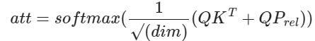
Relative Bias (T5)
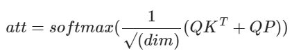
The T5 model, introduced by Raffel et al. in 2020, employs a technique known as "relative bias." Instead of using an embedding vector for each relative position, it utilizes a learnable scalar bias. This relative bias term is added to the corresponding logit during the computation of attention weights. This approach reduces the number of learned positional parameters, resulting in improved efficiency in terms of both memory and computation.
Mathematically, it can be expressed as:
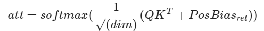
To further enhance efficiency, T5 shares the position embedding parameters across all layers in the model. However, within a given layer, each attention head utilizes a distinct learned position embedding. In our implementation, we employ relative bias for each unique relative position. It's important to note that the original T5 implementation used position binning, based on linear and logarithmic relative distances, to scale to larger contextual contexts.
Rotary Position Embedding (RoPE)
RoPE, introduced in RoFormer 2021, serves as the cornerstone of the LLama architecture and has found widespread adoption in other cutting-edge transformer models such as PaLM and Dolly. It revolutionizes the encoding of positional information for tokens by employing a rotation matrix. This matrix seamlessly incorporates explicit relative position dependencies into attention calculations. The RoPE rotation matrix offers remarkable flexibility, accommodating varying sequence lengths, diminishing inter-token dependencies as relative distances increase, and, notably, enhancing linear self-attention with relative position encoding.
The application of RoPE to Query (Q) and Key (K) vectors is elegantly simple. When you compute attention using the standard approach, it inherently infuses the result with relative position information:
q, k = self.rotary_emb.rotate_queries_and_keys(q, k)
# compute attention scores - Flash attention
out = torch.nn.functional.scaled_dot_product_attention(q, k, v, is_causal=True)
For a comprehensive understanding of its implementation, you can refer to the Colab section. For further exploration and insights, the eleutherAI Blog is an excellent resource. Additionally, you can access the official RoPE library and LLAMA Code Implementation.
One of the significant advantages of RoPE lies in addressing a key limitation of Relative Bias. Calculating relative positional bias, as done in T5, necessitates constructing a complete attention matrix for all pairs of positions in the input sequence. This operation has a quadratic time complexity, which is manageable for smaller input sequences but quickly becomes computationally intensive for longer ones. In this regard, RoPE shines, particularly when using efficient alternatives to softmax attention, including kernelized variants like FAVOR+, which don't require the computation of the full attention matrix.
Align and Bias (AliBi)

AliBi employs scalar bias values, similar to the Relative Bias technique. However, instead of learning these values, it derives them using a straightforward formula. The essence of AliBi lies in penalizing the attention assigned by a query to a key based on their relative distance. When a query and key are in close proximity, the penalty is minimal, but it significantly increases as they move farther apart.The biases decrease linearly in the log scale, and each head has a different slope. The slope calculation is as follows:
def get_slopes(n_heads: int):
    n = 2 ** math.floor(math.log2(n_heads))
    m_0 = 2.0 ** (-8.0 / n)
    m = torch.pow(m_0, torch.arange(1, 1 + n))
    if n < n_heads:
        m_hat_0 = 2.0 ** (-4.0 / n)
        m_hat = torch.pow(m_hat_0, torch.arange(1, 1 + 2 * (n_heads - n), 2))
        m = torch.cat([m, m_hat])

    return m
AliBi is very fast and is used in MPT. It was the first architecture to enable 100K context length. It outperforms Rotary embeddings in accuracy when evaluating sequences that are longer than the ones the model was trained on (extrapolation).
Landmark Attention

This is a recent attention mechanism emerging from Chinese AI research labs and has yet to be integrated into large foundational Language Model (LLM) architectures. Notably, it brings significant advancements to the attention mechanism, particularly when dealing with longer contextual information. AliBi and RoPE penalisation increases with relative position which heavily discourages the model to pick context information from large relative distance. Landmark-based approach solves this limitation. It employs a landmark token to represent the overall context of a block of text. It then leverages this landmark token to penalize the individual token attention. This innovative approach allows for efficient contribution of information from distant parts of a text block to the attention value.
I am curious to see its adoption in new LLMs. As this is more effective on longer context length, I have skipped the implementation here.
Evaluation and Comparison
Expanding upon our previous tutorial on Large Language Models (LLMs), we perform evaluations using the same tiny Shakespeare dataset. For educational purposes, I've created scaled-down versions of LLMs featuring 8 heads, 64 embedding dimensions, and a 32-token context. You're encouraged to give it a try; the training process requires only 10 minutes on Google Colab GPU. The figure below provides a comparative analysis of training parameters, as well as training and validation loss/perplexity performance.

As evident, AliBi boasts the fewest parameters, closely followed by RoPE. While the differences may appear relatively small in this context, they become more pronounced as you increase the context length from 32 tokens to 32,000 tokens or more. In our approach, Relative Bias, AliBi, and RoPE, all exhibit similar learning capabilities when considering the validation set perplexity. Importantly, this performance enhancement is achieved with the addition of only a minimal number of parameters. For a more detailed comparison, you can refer to the WandB experiment tracking dashboard.
What’s Next?
In this single post, we have successfully implemented scaled-down versions of T5 (decoder only), LLama, and MPT models from an architectural standpoint. To maintain simplicity for educational purposes, we've avoided some of the more complex optimizations. Still, it is powerful enough to showcase the effectiveness of recent relative position embedding evolution and where it is headed.
Next, we will take a look at several advancements that have been made in Efficient attention mechanisms such as Sparse Attention(BIG BIRD), FAVOR+ (Performer), MultiQuery Attention, and Longformer(Sliding Attention).
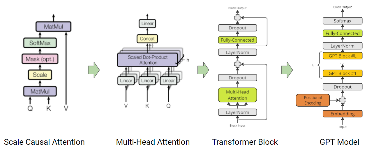
]]>In this post, we will code fundamental Transformer blocks, and embark on a journey to build a GPT model from the ground up. Our journey starts with Karpathy's guide on GPT from scratch - implementing tokenisation, self-attention, multi-head and causal attention, and trainable transformers. Building upon this foundation, we will further improve by introducing optimisation techniques like PreNorm, weight tying, flash attention, and merged QKV computation.
While this post introduces you to essential concepts with bits of code, you can seamlessly put these concepts into practice by following along with the linked Colab Notebook, which provides a step-by-step code implementation.
Hands-on Notebook: Github
Coding Transformer: The Fundamental Block
As introduced in the attention paper, Query (Q), Key (K) and Value (V) based efficient attention mechanism forms the core of the Transformer architecture. The attention mechanism calculates the output as a weighted sum of the values, where the weight assigned to each value is determined by the scaled dot-product of the query with all the keys. This allows the model to weigh the importance of each input token when making predictions.

Here’s an example of how attention can be implemented:
B, T, head_size = 4, 8, 64  # batch, token_context_length, head_size
k = torch.randn(B, T, head_size)
q = torch.randn(B, T, head_size)
v = torch.randn(B, T, head_size)

# Attention calculation
attention = torch.einsum('b t h, b s h-> b t s', q, k) * head_size ** -0.5
In Self-Attention, Q, K, and V are derived from a single input representation. On the other hand, in the domain of cross-attention, Q originates from one input, whereas K and V are extracted from another.
Casual-Attention
In addition to self-attention, decoder-based transformer models also use casual-attention. This type of attention masks future tokens to prevent the model from “cheating” by using information that is not available at the current time step. It is implemented by masking with the triangular matrix.
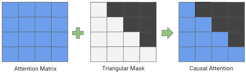
attention = attention.masked_fill(self.tril[:T, :T] == 0, float('-inf'))
attention = F.softmax(attention, dim=-1)
Multi-Head Attention
Multi-Head Attention capitalizes on the power of multiple heads to learn and calculate diverse attention patterns. This empowers the model to simultaneously focus on information from various representation subspaces at distinct positions. The following example illustrates how Multi-Head Attention module can be implemented with the causal attention mechanism:
class MultiHeadAttention(nn.Module):
    """ multi head of self-attention """

    def __init__(self, num_heads, head_size):
        super().__init__()
        self.num_heads = num_heads
        self.head_size = head_size

        self.key = nn.Linear(head_size, head_size, bias=False)
        self.query = nn.Linear(head_size, head_size, bias=False)
        self.value = nn.Linear(head_size, head_size, bias=False)
        self.register_buffer('tril', torch.tril(torch.ones(block_size, block_size)))

        self.dropout_wei = nn.Dropout(dropout)
        n_embd= num_heads*head_size
        self.proj = nn.Linear(n_embd, n_embd)
        self.dropout_proj = nn.Dropout(dropout)


    def forward(self, x):
        # Reshape the tensor to B N T H for N heads
        B,T,C = x.shape
        x = rearrange(x, 'B T (N H) -> B N T H', N=self.num_heads)

        k = self.key(x)   # (B,N,T,H)
        q = self.query(x) # (B,N,T,H)

        # compute attention scores \
        wei = torch.einsum("BNTH, BNSH -> BNTS", q,k) * self.head_size**-0.5
        wei = wei.masked_fill(self.tril[:T, :T] == 0, float('-inf'))
        wei = F.softmax(wei, dim=-1)
        wei = self.dropout_wei(wei)
        # perform the weighted aggregation of the values
        v = self.value(x) # (B,N,T,H)
        out = torch.einsum("BNTS, BNSH -> BNTH", wei, v)

        # concat and mix N Heads
        out = rearrange(out, 'B N T H -> B T (N H)')
        out = self.dropout_proj(self.proj(out))
        return out
Transformer Block
The building block of the transformer is crafted by fusing Multi-Head Attention with layer normalization, a non-linear MLP, and residual connections. Within a transformer-based Language Model (LLM), several layers of this foundational transformer block are used to capture intricate contextual relationships and produce cohesive output.
class TransformerBlock(nn.Module):
    """ Transformer block: communication followed by computation """

    def __init__(self, n_embd, n_head):
        # n_embd: embedding dimension, n_head: the number of heads we'd like
        super().__init__()
        head_size = n_embd // n_head
        self.sa = MultiHeadAttention(n_head, head_size)
        self.ffwd = FeedFoward(n_embd)
        self.ln1 = nn.LayerNorm(n_embd)
        self.ln2 = nn.LayerNorm(n_embd)

    def forward(self, x):
        x = x + self.sa(self.ln1(x))
        x = x + self.ffwd(self.ln2(x))
        return x
Implementing and Training mini-GPT model
Basic Bigram Model
Before we dive into the complexities of building a GPT, let’s start with the basics. A bigram model is a simple language model that predicts the next word in a sequence based on the previous word. Here’s an example of a BigramLanguageModel class:
class BigramLanguageModel(nn.Module):
    def __init__(self, vocab_size):
        super().__init__()
        # each token directly maps to the logits for the next token
        self.token_embedding_table = nn.Embedding(vocab_size, vocab_size)

    def forward(self, idx):
        # idx and targets are both (B,T) tensor of integers
        logits = self.token_embedding_table(idx) # (B,T,C)
        return logits

    def generate(self, idx, max_new_tokens):
        # idx is (B, T) array of indices in the current context
        for _ in range(max_new_tokens):
            # get the predictions
            logits, loss = self(idx)
            # focus only on the last time step
            logits = logits[:, -1, :] # becomes (B, C)
            # apply softmax to get probabilities
            probs = F.softmax(logits, dim=-1) # (B, C)
            # sample from the distribution
            idx_next = torch.multinomial(probs, num_samples=1) # (B, 1)
            # append sampled index to the running sequence
            idx = torch.cat((idx, idx_next), dim=1) # (B, T+1)
        return idx
This model can be used to generate text by predicting the next word in a sequence and then feeding that word back into the model to generate the next word. The colab notebook extends the above implementation with loss calculation and depicts simple generative LM training.
While a basic Bigram model can generate coherent text, it has its limitations. For example, it only considers the previous word when making predictions, which can result in repetitive or nonsensical text.
Decoder-based Transformer Model
To overcome the limitations of a basic Bigram model, we can use a decoder-based transformer model. This type of model uses self-attention to consider the entire input sequence when making predictions.
class TransformerModel(nn.Module):
    def __init__(self, vocab_size, n_embd, n_head, max_token_len, n_layer):
        super().__init__()
        # each token directly reads off the logits for the next token from a lookup table
        self.token_embedding_table = nn.Embedding(vocab_size, n_embd)
        self.position_embedding_table = nn.Embedding(max_token_len, n_embd)
        self.blocks = nn.Sequential(*[TransformerBlock(n_embd, n_head=n_head) for _ in range(n_layer)])
        self.ln_f = nn.LayerNorm(n_embd) # final layer norm
        self.lm_head = nn.Linear(n_embd, vocab_size)

    def forward(self, idx, targets=None):
        B, T = idx.shape

        # idx and targets are both (B,T) tensor of integers
        tok_emb = self.token_embedding_table(idx) # (B,T,C)
        pos_emb = self.position_embedding_table(torch.arange(T, device=device)) # (T,C)
        x = tok_emb + pos_emb # (B,T,C)
        x = self.blocks(x) # (B,T,C)
        x = self.ln_f(x) # (B,T,C)
        logits = self.lm_head(x) # (B,T,vocab_size)

        if targets is None:
            loss = None
        else:
            B, T, C = logits.shape
            logits = logits.view(B*T, C)
            targets = targets.view(B*T)
            loss = F.cross_entropy(logits, targets)

        return logits, loss
Optimizations
PreNorm
In PreNorm, the layer normalization is applied before the sublayer (e.g., self-attention or feed-forward) instead of after it, as in the original transformer model (PostNorm). GPT model already utilises PreNorm to provide better training stability.
Weight Tying
This method massively reduces the total number of parameters and improves the performance of language models by tying (sharing) the weights of the embedding and softmax layers. The intuition behind it is that both the embedding layer and the softmax layer learn word representations, such that similar words (in meaning) are represented by vectors that are near each other (in cosine distance). By sharing the weights between these two layers, the model can learn more efficiently and avoid overfitting.
# https://paperswithcode.com/method/weight-tying
self.token_embedding_table.weight = self.lm_head.weight
Flash Attention
The key idea behind Flash Attention is to make the attention algorithm IO-aware, meaning that it takes into account the reads and writes between different levels of GPU memory. Flash Attention uses tiling to load blocks of query, key, and value tensors from GPU high bandwidth memory (HBM) to SRAM (its fast cache). It then computes attention with respect to that block and writes back the output to HBM. By loading in blocks, Flash Attention is able to reduce the number of memory reads/writes between GPU HBM and GPU on-chip SRAM. This results in fewer HBM accesses than standard attention, making Flash Attention 7.5x faster and more memory-efficient.

In Torch 2.0, It can be simply utilised by using torch.nn.functional.scaled_dot_product_attention function. Refer colab section for transformer with flash attention.
Tokenizer
Up until now, we've employed a custom character-level tokenizer, requiring the model to decipher meaning character by character. To simplify this process for the model we can use more abstract units - words and sub-words. Just like, constructing a house is easier using bricks than working with individual grains of cement. However, this approach introduces a new challenge: a notable increase in the count of unique tokens (vocabulary). To address this, we incorporate subword tokenization to strike a balance.
from transformers import GPT2Tokenizer
tokenizer = GPT2Tokenizer.from_pretrained('gpt2')
input_text = "Your input text goes here."
input_ids = tokenizer.encode(input_text)
Typically, I opt for existing tokenization methods, which enable the utilization of pre-trained models. Nonetheless, the beauty of subword tokenization lies in its adaptability to domain-specific text. This is exemplified in the last colab section, where I demonstrate how subword tokenization can be tailored to custom content.
from tokenizers import Tokenizer
from tokenizers.models import BPE
from tokenizers.pre_tokenizers import Whitespace
from tokenizers.trainers import BpeTrainer

tokenizer = Tokenizer(BPE())
tokenizer.pre_tokenizer = Whitespace()
trainer = BpeTrainer(special_tokens=["[UNK]", "[CLS]", "[SEP]", "[PAD]", "[MASK]"])

tokenizer.train_from_iterator(text.split("\n"), trainer=trainer)
tokenizer.get_vocab_size()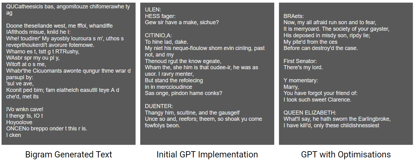
Our generated results significantly improve by integrating these optimizations into our training process for the mini GPT model, even with just 1 million parameters. It's worth noting that state-of-the-art (SOTA) GPT models scale up to sizes exceeding 100 billion parameters, achieving even lower perplexity and more advanced generative capabilities. Nevertheless, despite these scaling differences, the core principles and fundamentals underlying the architecture remain consistent.
What's Next?
Several advancements have been made to improve the capabilities and efficiency of transformer models:
- Integrated Positional embeddings - Fixed, Relative PE (T5), RoPe (llama), AliBi
- Attention optimisations - Efficient attention mechanisms such as Sparse Attention(BIG BIRD), FAVOR+ (Performer), MultiQuery Attention, and Longformer(Sliding Attention).
- Feedforward Network - Optimisations use of CNNs, routing mechanisms
- Training Data - Proper preprocessing and cleaning of training datasets
In our upcoming blog post within this series, our focus will shift towards exploring enhancements related to positional embeddings. Stay tuned and don't hesitate to connect with me on LinkedIn for further discussions.
]]>The advent of "Attention Is All You Need" by Vaswani et al. in 2017 marked a monumental milestone in the development of Language Models (LLMs). It revolutionized language processing with its Transformer Architecture based on a novel MultiHead Attention Mechanism (Q, K, V). It further provided a practical bidirectional encoder, the iterative decoder and the causal decoder architectures to efficiently solve NLP use cases. Andrej Karpathy's Let's build GPT: from scratch video fundamentally showcased the power of the same transformer in recent large language models. This video inspired me to consolidate further developments in transformer architectures in recent LLMs via code. Let's embark on a journey into the world of modern LLMs with a conceptual introduction and explore their transformative capabilities.
We will cover:
- The Transformer: A Fundamental Building Block
- Evolution of Transformers
- Pretraining: Unlocking Language Knowledge
- Emergence and Applications
- Alignment: Ensuring Ethical and Human-Aligned Behavior
- Finetuning: Domain-Specific Adaptation
The Transformer: A Fundamental Building Block
At the core of modern LLMs lies the Transformer architecture. The attention paper introduced the following key components:
- Efficient Attention Mechanism: Introduced Q, K, V attention mechanism enabling parallelization and scalability, with techniques like scaling and softmax for optimal attention distribution. MultiHead attention enhanced model performance.
- Transformer Architecture: Good model architecture with position encoding, Multi-Head attention, layer norm, MLP-based non-linearity, and residual connections. Efficient for optimizing large models.
- Encoder Architecture: Efficient bidirectional transformer architecture to consume and encode information into embedding space.
- Decoder Architecture: Iterative decoding architecture generates natural text step by step. It can also utilize encoded encodings for guidance, enhancing capability and quality.
- Causal Decoder: Efficient unidirectional decoder packing multiple sentence variations into a single batch, improving training efficiency.

The attention mechanism calculates the output as a weighted sum of the values, where the weight assigned to each value is determined by the scaled dot-product of the query with all the keys:

Multi-head attention allows the model to jointly attend to information from different representation subspaces at different positions. Finally, Multi-Head attention is integrated with layer norm, MLP-based non-linearity, and residual connections to form the transformer block. The transformer-based versatile Encoder-Decoder model enables LLMs to excel in various language tasks such as machine translation and text generation, thanks to its ability to capture contextual dependencies and generate coherent output. Overall, these components provided three fundamental advantages to transformers to revolutionise the AI roadmap:
- Expressiveness: A generic architecture allows it to capture intricate language patterns and semantics. It can capture global context, learn long-term dependencies in sequences and can also scale across modalities.
- Parallelization: Transformers can process input sequences in parallel, unlike sequential models like RNNs. It enables faster training and inference of larger models on large datasets and larger input contexts.
- Optimization: Finally, the transformer architecture with layer norm and residual connections provides the ability to train deep models capable of showcasing emergent behaviours.
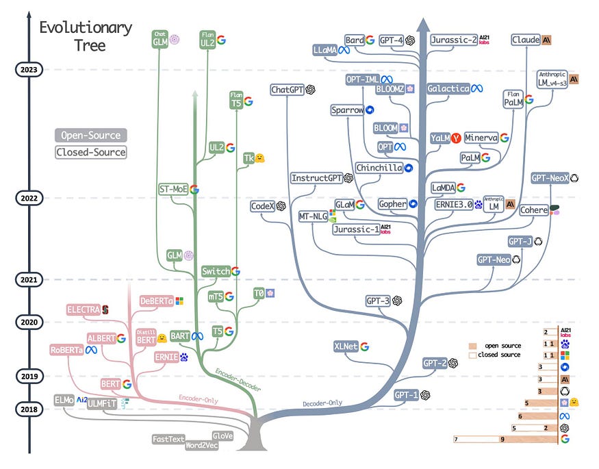
Evolution of Transformers
The first evolution of LLMs happened in model architecture from Encoder-Decoder to Encoder-only, Decoder-only, and prefix decoders.
- Encoder-Decoder: Traditional encoder-decoder architecture. BART, T5, FlanT5.
- Encoder-only: Consists of only the Encoder part of the Transformer architecture. Adept at capturing contextual representations of input sequences and have been extensively used in various embedding models. BERT, MiniLM etc.
- Decoder-only: Most successful architecture in scaling language generation tasks. iteratively next-word generation makes the task easier and causal decoder makes training efficient. GPT-series, OPT, llama, BLOOM etc.
- Prefix Decoders: It utilizes a bidirectional attention mechanism to encode the prefix and decodes the rest of the output tokens autoregressively using causal attention. PaLM.
A causal decoder has the advantage of spreading the computational and cognitive load by generating one word at a time. For example, for generating a text containing 100 words (tokens), the model will perform 100 passes and will be able to utilise 100x computing with the same parameters. This simplifies the task and improves the performance. Similar examples of improving capabilities by spreading cognitive and computing load are also manifested in other domains. In Image generation, the diffusion models also leverage similar strategies to outperform GAN models. However, similar to GigaGAN, scaling of the model and training of encoder models can also lead to an equally capable and more efficient inference. With further improvement in computing, more architectures similar to prefix decoders will emerge.
Another evolution happened within the transformer block to improve the capabilities and efficiency. Some of the notable ones are:
- Integrated Positional embeddings - Fixed, Relative PE (T5), RoPe (llama), AliBi (MPT)
- Attention optimisations - Efficient attention mechanisms such as Sparse Attention(BIG BIRD), FAVOR+ (Performer), MultiQuery Attention (Falcon), and Sliding Attention (Longformer).
- Feedforward Network - Optimisations use of CNNs, routing mechanisms
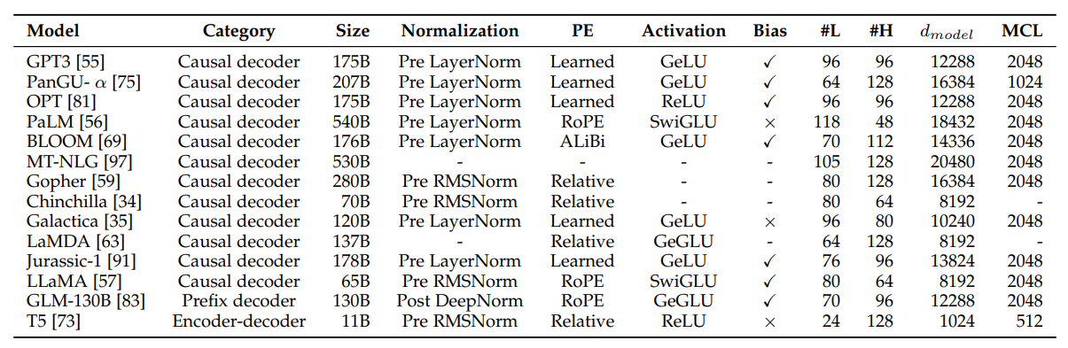
A Survey of Large Language Models paper succinctly summaries the significant LLM model architecture in a table:

Pretraining: Unlocking Language Knowledge
The pretraining phase is the initial step in the development of modern LLMs, where the model learns from a massive amount of text data without specific task supervision. Training objectives involve either predicting the next word/token(causal decoders) or predicting missing words in a given context. The other objective is also known as "masked language modelling," where a certain percentage of tokens in the input sequence are randomly masked, and the model is tasked with predicting those masked tokens based on the context. This unsupervised learning process allows the model to gain a deeper understanding of language and form a strong word representation which led to the emergence of intelligence.
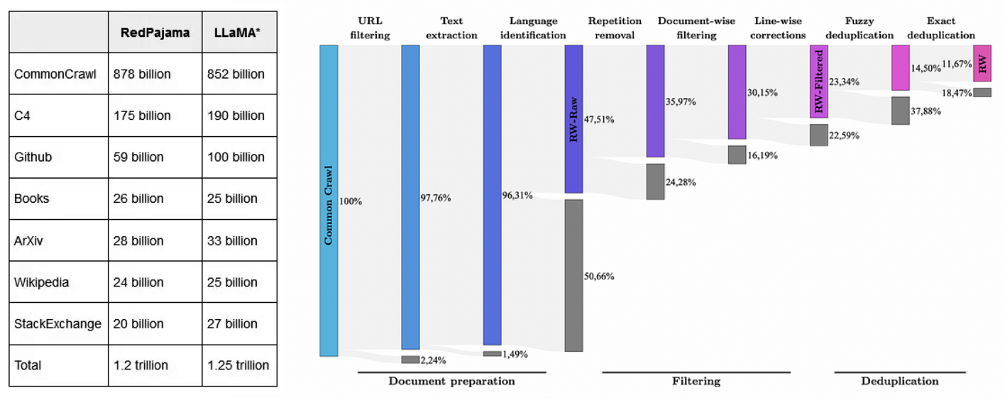
The size and quality of the training dataset are very essential for generating good-quality LLM. Scaling laws provides a relationship between optimal dataset requirements for a large model for optimal training [calc]. Smaller models can still be trained on bigger datasets but with diminishing returns. In today’s LLMs, the pretraining is performed on a trillion token scale dataset aggregated from the web, books, wiki, GitHub and other sources. Llama and RedPajama were pre-trained on 1.2T tokens. Falcon improved the performance over Llama and RedPajama by refining the collected dataset through multiple stages of filtering. Llama 2 further improves the base performance by training on 2 trillion tokens. The fineweb-Edu dataset further improved training efficiency.
While training objectives are usually simple, the dataset and model size requires a different scale of infrastructure to support large-scale pretraining. It usually incorporates 250-2048 GPUs and costs around 1-10M USD to train 10 billion parameter scale models. Bloom's blog is a good read on what goes behind a large-scale pretraining infrastructure. Also, simons blog provides good estimates.
Emergence and Applications
Emergent properties in language models highlight an intriguing phenomenon: as the number of parameters increases, performance initially fluctuates randomly until reaching a critical threshold. At this point, a distinct property emerges, leading to a remarkable improvement in performance. Despite a lack of complete understanding of this phenomenon, the "World model" hypothesis suggests that predicting the next word effectively requires learning to model the world. As the number of parameters increase, these models develop more comprehensive representations of human knowledge and language, essentially forming these mini “world models”. This critical juncture empowers the models with a heightened understanding of human language and enables contextually nuanced responses. As a result, they become valuable assets across various applications, including language translation, text generation, and interactive virtual assistants.

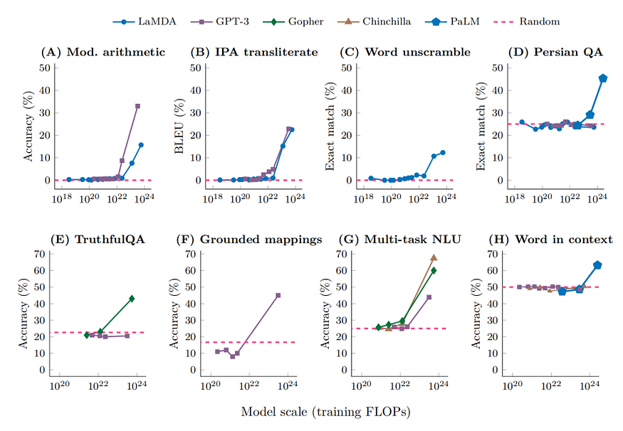
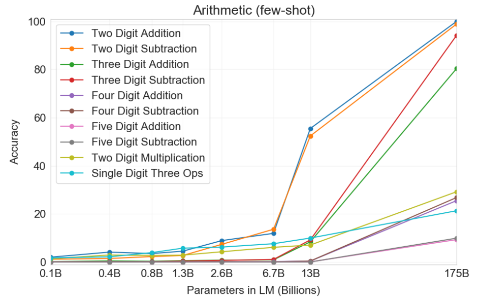
Emergent abilities of large language models. Image Source
Alignment: Ensuring Ethical and Human-Aligned Behavior
Pretrained LLMs may exhibit intelligent behaviour, but their training to predict the next word on vast internet text can also lead to generation outputs that are untruthful, toxic, or reflect harmful sentiments. In other words, these models' outputs aren’t aligned with their users' desired behaviour. Also, user-aligned behaviour is not enough. A user might ask to kill another human or a terrorist group might utilise the LLM intelligence for malicious purposes. This leads to the requirement of safety and ethics in AI. As we are rapidly progressing towards superintelligence, alignment becomes even more crucial.
To address human alignment, OpenAI introduced reinforcement learning from reinforcement learning from human feedback (RLHF) technique. Additionally, for a more robust embodiment of human ethics principles, Claude utilizes constitutional AI to make it safer and interpretable.

Finetuning: Domain-Specific Adaptation
Fine-tuning adapts pre-trained models to specific tasks or domains using smaller labelled datasets. During pretraining, LLMs gain a comprehensive understanding of language and accumulate a vast knowledge base. The transformer models transfer their general language knowledge to new tasks, demonstrate domain generalization capabilities, and deliver improved performance on downstream tasks, all with the utilization of only limited labelled data. This two-step approach empowers LLMs to excel in a wide range of practical applications, showcasing their adaptability and versatility.
Galactica uses a mixing of pretraining data with finetuning data to unlock alignment without harming base transformer capabilities. Orca's progressive learning is driven by careful sampling and selection of extensive and diverse imitation data. This data is further enriched by incorporating valuable signals from GPT-4, such as explanation traces, step-by-step thought processes, and complex instructions. LIMA by Meta also uses a 65B parameter LLaMa language model fine-tuned with the standard supervised loss on only 1,000 carefully curated prompts and responses, without any reinforcement learning or human preference modelling to provide a competitive model.
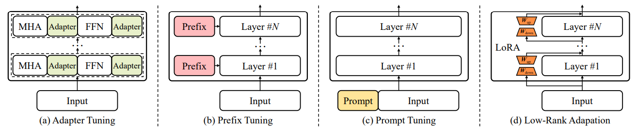
Due to the large scale of LLMs, Fine-tuning is also very costly. It leads to the emergence of Parameter-Efficient Fine-Tuning (PEFT) methods to enable efficient adaptation of pre-trained language models to various downstream applications by only fine-tuning a small number of (extra) model parameters. These are also often utilised to distil larger and more intelligent models into smaller models. However, The False Promise of Imitating Proprietary LLMs showcases that there exists a substantial capabilities gap between open LM using PEFT techniques and closed LMs. Vicuna like open LMs easily copy persona from chatGPT/GPT4 but they significantly lack base reasoning and factuality capabilities.
What's Next?
In our upcoming blog, we will embark on an exciting journey of coding a transformer model inspired by Karpathy's tutorial. Taking it a step further, we will implement optimizations such as weight tying, flash attention, and other enhancements to create an even more powerful and efficient model.
]]>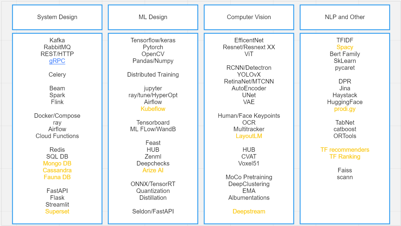
Here are some of the go-to ML tools that I find extremely useful for computer vision applications.
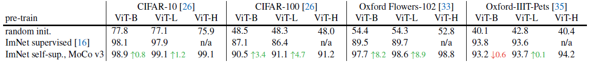
Contrastive methods currently achieve state-of-the-art performance in self-supervised learning. It not only enables learning from unlabeled data but even pushes accuracies for supervised learning and search-retrieval tasks. AI giants like Google, Meta, OpenAI are actively working and publishing new methods in the fields to improve Self-supervised learning. It also happens to be my recent work and research interest. I will introduce some fundamentals of contrastive learning here to build understanding. In the next post, we will cover the progress we have made.
We will cover:
- Representation learning methods
- Ingredients of Contrastive Learning
- Applications
- Implementations - ML Libraries and Resources
Representation learning methods
There are three prominent self-supervised representation learning methods: generative, multi-task modelling, and contrastive. Generative representational learning approaches use autoencoder or adversarial learning to learn latent embedding space for regenerating images. As Generative methods typically operate directly in pixel space and require a high level of detail for image generation. This makes it computationally expensive, and bigger model size, which may not be necessary for representation learning.
Multi-task modelling is also a very powerful method for representation learning. It involves joint embedding space by performing multiple tasks such as classifications, detection, translation etc. It is being used in state-of-art big language models. However good task selection is very important. Otherwise, there may be suboptimal performance in unrelated tasks.
Contrastive methods currently achieve state-of-the-art performance in self-supervised learning. Contrastive approaches avoid a costly generation step in pixel space by bringing the representation of different views of the same image closer (‘positive pairs’) and spreading representations of views from different images (‘negative pairs’) apart.
Ingredients of Contrastive Learning
A few of fundamentals for contrastive learning are creating positive and negative pairs, using a proper distance measure to measure embedding distance, defining a good training objective which can optimise the distance, using a good model architecture to learn representations and then using good learning strategies for optimal flow of loss gradients for model learning. Let’s dive a little bit deeper into each aspect:
Positive and Negative Dataset
To perform contrastive learning, you need to positive and negative pairs. How they can be created depends upon whether the dataset is labelled or un-labelled. For labelled datasets, all images belonging to same class consist of positive pairs and from different classes as negative pairs. For unlabelled datasets, positive pairs are created via augmentation of same image and augmentation of different images constitutes negative pairs.
The amount of positive and negative samples is also very important. Siasemes Network used just a pair of images, positive and negative alternatively. Triplet Loss improved by using 3 images - anchor, positive and negative. Most of today’s state-of-art methods use multiple positive and negative samples. Larger the sample size, more information the model will have about the features it needs to bring closer or pull apart. For example, researchers from MoCo v3 presented that a negative sample size of 4000 is the optimal size for imagenet dataset.
If the negative sample size is smaller, hard negative mining can be used to find the most effective negative samples. It significantly speeds up the training. However negative hard mining is more effective in labelled data. In the case of unlabelled or noisy labelled data, hard negative mining results in the degradation of performance. Some recent work (BYOL, SwAV, VICReg, SimSiam) even showcase that just using positive samples yields better results, removing the need for negative samples altogether. However, these methods require longer training time.
Augmentation used in state-of-art methods for positive samples has converged to the combination of weak and strong augmentation from the SIMCLR method. One positive sample is generated through weak augmentation and another via strong augmentation. Then strongly modified image representation is used to bring closer to weakly modified representation.
Distance Measure
How the distance of two representation vectors is measured, directly affects the representation space learning. Some popular distance measures which can be used are Euclidian distance, cosine similarity, manhattan distance, KL divergence, JS divergence, Wassertain (EM) distance. Each of them imparts special properties to representational space. So choosing an appropriate distance measure is important.
Training objective
It calculates the final loss value using the distance of provided positive and negative sample. This loss value is used to optimise the model. Some of the popular loss functions are -
- Contrastive loss (Siamese loss)
- Triplet loss
- N-pair loss
- Lifted Structured Loss
- NCE and InfoNCE Loss
- Circle Loss
- Soft Nearest Neighbor Loss
- VICReg Loss
- SigLIP and SigLIT
Network Architecture
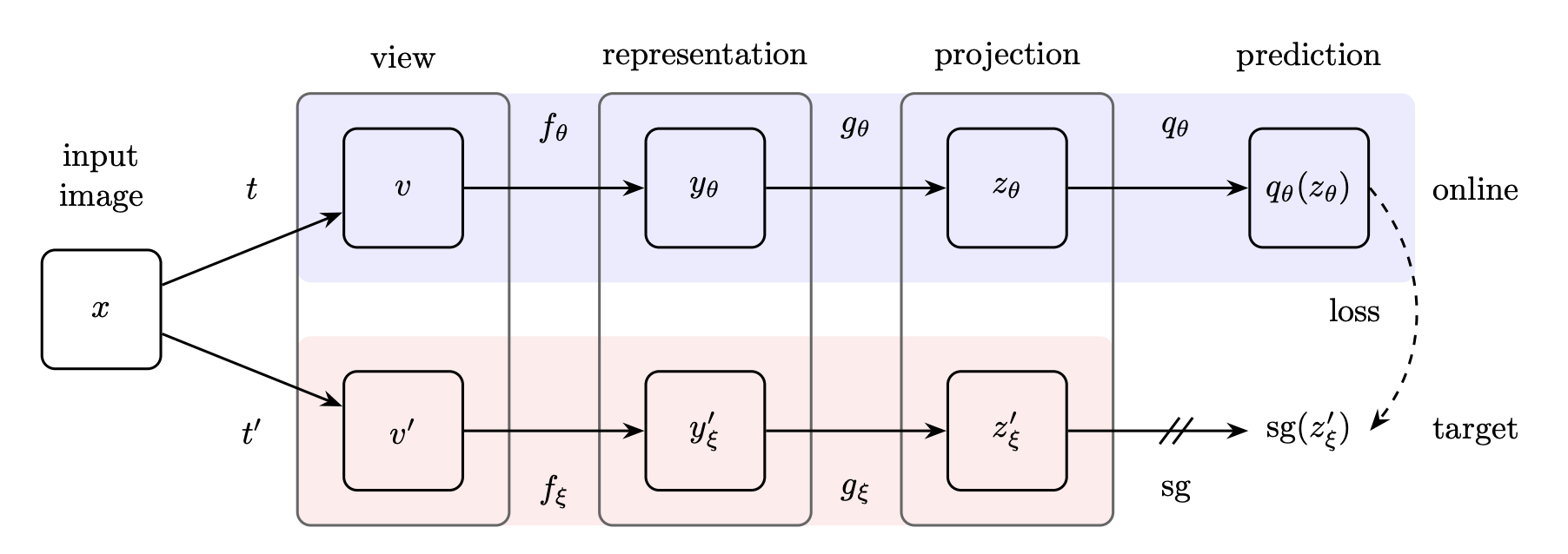
State-of-art methods use four-layer network architecture for contrastive learning - backbone model (view), representation layer, projection layer and prediction layer. Representation layer provides higher dimensional representation space, which can be used as input to the classifier or other downstream tasks. Projection layer is a lower dimension representation space which can be used for similarity measures. Prediction layer not only prevents collapse by providing asymmetry but also encourages the network to find features which are consistent between layers. Some approaches drop the prediction layer.
Learning Strategies
Grads Flow
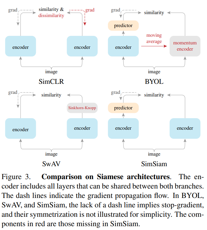
EMA
MoCo and BYOL models use EMA or momentum for target weight updates. It brings stability to representational space.
Target Temperature
In the case of a teacher-follower arm setup, teacher projection can be sharpened or the follower can be smoothened. It improves the feature sharpness of student.
Applications
Again, first, we should cover where it should not be used. It should not be the first step towards model/representation building. The use of pre-trained models via transfer learning is always a good start. There are some applications where it shines:
Label efficient training (one-shot/few-shot) - Self-supervised learning lets the model harness the power of unlabelled data to learn representation space. Linear evaluation or KNN-based methods in one or few shot provides significant results. It can further be used either finetuning with small labelled dataset or as a backbone for multiple classifiers on top. I can think of typical factory or medical oriented usecases where there is less labelled data or pre-trained model access and you need to work on multiple usecases. Here collecting large raw dataset is easy but building a well-labelled dataset not only requires experts for labelling but also is a challenging task.
Pretraining - Self-supervised achieves better results than transfer learning on pre-trained models even in fully labelled dataset availability.
Search and retrieval - Projector layer provides a really good feature vector to be used for search and retrieval of similar item search.
Implementations - ML Libraries and Resources
If you are in the TensorFlow ecosystem then TensorFlow Similarity is a really good option. It provides self-supervised learning on both labelled and unlabelled data, lets you control representation, projector and predictor layer configurations and have most state-of-art loss function implementations such as TripletMarginLoss, SoftNearestNeighborLoss etc.
Pytorch Metric Learning is a good library in the PyTorch ecosystem for labelled and unlabelled datasets. It also provides state-of-the-art loss functions, distance measures and miners for hard negative mining.
If you are a researcher, you can also look into official repositories. These are also well organised. I prefer this method more if I want to tweak and try out some new ideas.
Thank you for reading. There are some good references for further knowledge grasp:
- Review Blog — MoCo v3: An Empirical Study of Training Self-Supervised Vision Transformers
- Good Knowledge Blog - Contrastive Representation Learning, Lilian Weng
- Practical Insights Paper - Rethinking Self-Supervised Learning: Small is Beautiful
Deep neural networks have many tunable hyperparameters which need to be selected to get maximum accuracy out of your datasets and models. It can be used to find the best neural architecture (NAS) by
]]>TLDR; Use Ray Tune or NNI, they provide SOTA algorithms out of box for efficient HPO.
Deep neural networks have many tunable hyperparameters which need to be selected to get maximum accuracy out of your datasets and models. It can be used to find the best neural architecture (NAS) by optimising layer choice, number of layers, and layer width, or finding the best learning algorithm by optimising learning rate, momentum, optimizer choice, data augmentation etc.
We will cover:
- When to use HPO
- How HPO works
- State-of-art HPO algorithms
- How to use - Ray Tune and NNI
When to use HPO
First, let’s cover where to not use HPO. If you have a dataset similar to pre-trained datasets and you are not hunting for last 3-4% accuracy gains, you should not use HPO. It will consume 10x more resources and time for such gains. In my experience, good authors or libraries provide good default values which are a result of both intensive HPO and domain expertise. Also, model architecture HPO should not be a primary way to optimize performance w.r.t accuracy for standard problems. There is a wider range of network architectures and sub-architectures available that trade accuracy for performance. For example, in vision classification, you can use architectures from VIT to EfficientNet to MobileNet and small, medium, large sub-architecture within. They provide 10-100x performance gain with a tradeoff of 3-10% accuracy. Optimisation techniques are the next best choice. However, HPO can also be used for the evaluation of all these choices.
But if you are an academic user, where a 1-2% gain is a SOTA decision maker or 3-4% improvement has a significant impact on business, then HPO is a really good choice. HPO provides very good results if the standard model and configurations are not yielding good results. It shines when you dwell in no-man’s land such as new algorithm development or custom model architecture design. Tuning large parameters manually is impossible with high complexity scenarios. I have used this to design custom model architecture that provides 10x performance while retaining accuracy for specific segmentation tasks.
How HPO works
HPO consist of two parts - search algorithm and scheduler. Search algorithm selects hyperparameter value for a trial from complete parameter space and scheduler decides the run duration or resource allocation to trial.
Two basic search algorithms are grid search and random search. Random search works better than grid search. It is also the best choice for embarrassingly parallel optimisation. One state-of-art search algorithm is Bayesian Optimisations. It utilizes surrogate bayesian model on search space to efficiently find optimal values. It can select value based on maximum uncertainty (exploration) or maximum gain (exploitation) from bayesian modelled search space and then improve search space modelling based on trial results. Two major drawbacks are that this algorithm in its naïve form is not parallel (next value selection is dependent on current value evaluation) and it only supports continuous values. However advanced implementations such as TPE and BOHB address these limitations.


A naive scheduler runs all trails for complete durations and evaluates them after. Successive halving or Asynchronous Successive halving (ASHA) keeps the best halves of the trials and discards half of the trials that are not good. It will continue until we have just one single configuration. It optimises resource allocation to good trials, resulting in faster training. Hyperband scheduler further improves upon this by starting new configuration trials in place of discarded trials. This increases the number of trials evaluated, resulting in better hyperparameters. ASHA or Hyperband requires that all configurations can be stopped early and validation score can be obtained.

State-of-art methods such as BOHB, combining bayesian optimisation and hyperband can lead to 5-20x speed up on HPO.

State-of-art HPO algorithms
How to use - Ray Tune
Ray Tune is a really good tool for HPO. It is simple and powerful. As part of Ray ecosystem, it is scalable to multi-GPU and distributed environments. It provides all the above and additional SOTA algorithms. You can find more details here. Microsoft NNI is also a really good choice if you are using PyTorch ecosystem. It is even better for NAS use cases. But its support for non-PyTorch frameworks is limited.
HPO with Bayesian optimisation and HyperBand scheduler can be quickly implemented in Ray Tune via the following reference:
from ray import tune
from ray.tune.search.hyperopt import HyperOptSearch
from ray.tune.search import ConcurrencyLimiter
from ray.tune.schedulers import AsuncHyperBandScheduler
from ray.air import session


# 1. Define an objective function.
def trainable(config):
   #import torch/keras -        import pytorch/tf/keras here if using, known issue with GPU trials

    for x in range(20):  # "Train" for 20 epoch.
        one_epoch_training(model, config["lr"], config["a"])
        accuracy = calc_accuracy(model)
        session.report({"accuracy": accuracy})  # Send the score to Tune.

# 2. Define a search space.
search_space = {
   "lr": tune.loguniform(1e-8, 1e-2, base=10),
   "a": tune.choice([1, 2, 3]),
}


# 3. Define Search Algo and Scheduler
search_algo = HyperOptSearch()
search_algo = ConcurrencyLimiter(search_algo, max_concurrent=4) # Limit concurrent trials since BO doesn't parallelize very well

scheduler = AsuncHyperBandScheduler(metric="accuracy", mode="max", grace_period=5)

# 4. Start a Tune run that maximizes accuracy.
tune_config = tune.TuneConfig(
    search_alg=search_algo,
    metric="accuracy", mode="max",
    num_samples= 20 # Number of trials
)

tuner = tune.Tuner(
    trainable,
    tune_config= tune_config,
    param_space=search_space,
    scheduler = scheduler
)

results = tuner.fit()
print(results.get_best_result(metric="score", mode="min").config)
This should get you started on journey of optimizing hyperparameters efficiently with state-of-art algorithms. Combining with techniques like µTransfer makes it even more promising. OpenAI fine-tuned a 40 million parameter proxy GPT3 model before transferring the optimal hyperparameters to the 6.7B parameter variant. With only a 7% extra training budget for hyperparameter search, it outperformed the 13B variant. To learn more about this, these are some good references:
- Ray Tune: https://docs.ray.io/en/latest/tune/key-concepts.html
- Good blogs to take reference: Blog 1 , Blog 2
- FLAML: https://github.com/microsoft/FLAML
- Fabolas: https://arxiv.org/abs/1605.07079
- PBT: https://www.deepmind.com/blog/population-based-training-of-neural-networks and https://www.deepmind.com/publications/faster-improvement-rate-population-based-training
- µTransfer: https://decentdescent.org/tp5.html